what is Scrum-Introduction to Scrum

Introduction to Scrum 

Continuous Process Improvement

“Release Plan” for this Session

Intro to Agile

Intro to Agile-Myths and Facts

Agile Principles & Values

We are uncovering better ways of developing software by doing it and helping others do it. Through this work we have come to value

Agile Principles..

Principle #1 Our highest priority is to satisfy the customer through early and continuous delivery of valuable software.
Principle #2 Welcome changing requirements, even late in development. Agile processes harness change for the customer's competitive advantage.

Principle #3 Deliver working software frequently, from a couple of weeks to a couple of months, with a preference to the shorter timescale.

Principle #4 Business people and developers must work together daily throughout the project.

Principle #5 Build projects around motivated individuals. Give them the environment and support they need, and trust them to get the job done.

Principle #6 The most efficient and effective method of conveying information to and within a development team is face-to-face conversation.

Principle #7 Working software is the primary measure of progress.

Principle #8 Agile processes promote sustainable development. The sponsors,

developers, and users should be able to maintain a constant pace indefinitely. 

Principle #9 Continuous attention to technical excellence and good design enhances agility.

Principle #10 Simplicity--the art of maximizing the amount of work not done--is essential.

Principle #11 The best architectures, requirements, and designs emerge from self organizing teams.

Principle #12 At regular intervals, the team reflects on how to become more effective, then tunes and adjusts its behavior accordingly.

Let’s Set the Stage….

1. Time Boxing : An act of putting Strict Time boundaries around an Action or Activity.
2. Sprint : In Scrum, Work is always done in regular repeatable work cycle known as Sprint.  Sprint is an iteration with fixed time box.

3. Velocity: is a measure of the amount of work a Team can tackle during a single Sprint and is the key metric in Scrum. Velocity is calculated at the end of the Sprint by totalling the Points of all fully completed User Stories. 

4. Scrum : Scrum is an Agile way of doing Projects usually Software Development but not limited to. It provides a lightweight process framework that embraces iterative and incremental practices, helping organizations deliver working projects more frequently.

Scrum Roles

Product Owner.

1. Responsible for maximizing the value of the product and the work of the Development Team. 

2. Creates and maintains the Product Backlog.

3. Prioritizes and sequences the Backlog according to business value or ROI.

4. Assists with the elaboration of Epics, Themes and Features into user stories that are granular enough to be achieved in a single sprint.

5. Represents the customer, interfaces and engages the customer.

6. Terminates a Sprint if it is determined that a drastic change in direction is required.

7. Inspects the product progress at the end of every Sprint and has complete authority to accept or reject work done.

Scrum Master.

1. Responsible for ensuring Scrum is understood and enacted

2. Responsible for enacting Scrum values and practices.

3. The Scrum Master serves the team (helping them remove any and all impediments 

that surface), protects the team (from any outside disruption or interference), and teaches and guides the team’s use of Scrum.

4. Gathers support from everyone to make sure that the change is accepted.

5. Train, mentor and make the team speak the same language.

6. Protects the team from the outside interference.

7. Unblocks impediments so that the team can achieve the sprint goal.

Scrum Team (Team).

1. Collectively responsible for converting product backlog into product increment.

2. Self-organizing. Self-Organize to collectively deliver product increment every sprint

3. A cross-functional team. Understand and commit to sprint goal. Create sprint backlog. Create Just enough design for the sprint goal

4. Understand the User stories, estimate them , break the stories in task etc..

5. Understand the product vision & help each other in achieving committed  Sprint goal.

6. Demonstrate the work done and understand both verbal and non-verbal feedback.

7. Actively participate in Retrospective and identify process improvements to get better at delivering value

Scrum Team- The Ultimate Responsibility

Scrum-Values.

A Good Product Backlog is.

Sprint Backlog.

1. The Product Backlog items selected for this Sprint + the plan for Delivering them is Sprint Backlog

2. During the sprint planning meeting, the team selects some number of product backlog items, usually in the form of user stories, and identifies the tasks necessary to complete each user story is Sprint Backlog.

Product Increment.

1. The Increment is the sum of all the Product Backlog items completed during a Sprint and the value of the increments of all previous Sprints.

2. At the end of a Sprint, the new Increment must be “Done,” which means it must be in useable condition and meet the Scrum Team's definition of “Done.”

Backlog Grooming ( Product Backlog Refinement )

It is the act of adding detail, estimates, and order to PBI.

It’s a part-time activity during the sprint and how and when is decided by the Scrum Team.On going process of collaboration between PO and the Development Team

Sprint Planning Meeting

1. Takes place before the start of every Sprint

2. Attended by Team, Product Owner, Scrum Master, Stakeholders

3. The product owner presents the ordered PBIs to the Development Team.

4. The Development team Pulls and discuss PBIs, ask clarifying questions and understand the acceptance criteria. Select the PBI for Sprint. 

5. Continue step 4 until Sprint backlog is full.

6. The Scrum team crafts the sprint goal.

7. Team understands the details of what the Product Owner has prioritized on
the Product Backlog

8. Team decides how much productive time it has available during the Sprint.

9. Team decides how many Product Backlog items it can commit to complete during
the Sprint.

Sprint Planning.

Daily Stand up Meeting.

Daily Stand up Meeting.

DSM: The Agreement & The Protocol

Scrum Values and DSM.

Scrum Framework

Sprint Review Meeting.

1. At the end of the Sprint, the Product Owner, Team, Scrum Master, and Stakeholders come together and see a demo of what the team has produced.

2. Attended by Team, Product Owner, Scrum Master, Stakeholders.

3. The Development Team Demonstrates the work done to the PO and Other Stakeholders.

4. PO verifies things and accepts or rejects the work done.

5. Development team discusses how the last Sprint went.

6. PO identifies the work done and what has not been done.

7. The Purpose is to Inspect the product increment and adapt the product backlog.

8. PO gives feedback to the team and updates the Product Backlog.

Sprint Review Meeting.

Sprint Retrospective Meeting.

1. Inspect how last sprint went with regards to people, relationship, process, and tools

2. Attended by Team, Product Owner, Scrum Master.

3. This is the mechanism for continuous improvement where critical problems are identified and addressed.

4. The Team, Product Owner, and Scrum Master meet at the end of each Sprint to review their way of working, and look for ways to improve their effectiveness.

5. Primary Objective of this Meeting is to identify 

3 specific items.

1. Things the team needs to keep doing : ---- Best practices

2. Things the team needs to begin doing: ---- Process Improvements

3. Things the team needs to stop doing : ---- Process Problems and Bottlenecks

Sprint Burn Down Chart.

Release Burn Down Chart.

Thank You

Restfull web services

Merge sort Analysis and Alorithem

A sorting algorithm based on divide and conquer. Its worst-case running time has
a lower order of growth than insertion sort.
Because we are dealing with subproblems, we state each subproblem as sorting
a subarray A[p . . r ]. Initially, p = 1 and r = n, but these values change as we
recurse through subproblems.
To sort A[p . . r ]:
Divide by splitting into two subarrays A[p . . q] and A[q + 1 . . r ], where q is the
halfway point of A[p . . r ].
Conquer by recursively sorting the two subarrays A[p . . q] and A[q + 1 . . r ].
Combine by merging the two sorted subarrays A[p . . q] and A[q + 1 . . r ] to produce
a single sorted subarray A[p . . r ]. To accomplish this step, we’ll deÞne a
procedure MERGE(A, p, q, r ).
The recursion bottoms out when the subarray has just 1 element, so that it’s trivially
sorted.
MERGE-SORT(A, p, r )
if p < r Check for base case
then q ← (p + r)/2
Divide
MERGE-SORT(A, p, q) Conquer
MERGE-SORT(A, q + 1, r ) Conquer
MERGE(A, p, q, r ) Combine
Initial call: MERGE-SORT(A, 1, n)
[It is astounding how often students forget how easy it is to compute the halfway
point of p and r as their average (p + r)/2. We of course have to take the ßoor
to ensure that we get an integer index q. But it is common to see students perform
calculations like p +(r − p)/2, or even more elaborate expressions, forgetting the
easy way to compute an average.]
Example: Bottom-up view for n = 8: [Heavy lines demarcate subarrays used in
subproblems.]



[Examples when n is a power of 2 are most straightforward, but students might
also want an example when n is not a power of 2.]
Bottom-up view for n = 11:



Merging

What remains is the MERGE procedure.

Input: Array A and indices p, q, r such that

• p ≤ q < r .

• Subarray A[p . . q] is sorted and subarray A[q + 1 . . r ] is sorted. By the

restrictions on p, q, r , neither subarray is empty.

Output: The two subarrays are merged into a single sorted subarray in A[p . . r ].

We implement it so that it takes (n) time, where n = r − p + 1 = the number of

elements being merged.

What is n? Until now, n has stood for the size of the original problem. But now

we’re using it as the size of a subproblem. We will use this technique when we

analyze recursive algorithms. Although we may denote the original problem size

by n, in general n will be the size of a given subproblem.

Idea behind linear-time merging: Think of two piles of cards.

• Each pile is sorted and placed face-up on a table with the smallest cards on top.

• We will merge these into a single sorted pile, face-down on the table.

• A basic step:

• Choose the smaller of the two top cards.

• Remove it from its pile, thereby exposing a new top card.

• Place the chosen card face-down onto the output pile.

• Repeatedly perform basic steps until one input pile is empty.

• Once one input pile empties, just take the remaining input pile and place it

face-down onto the output pile.

• Each basic step should take constant time, since we check just the two top cards.

• There are ≤ n basic steps, since each basic step removes one card from the

input piles, and we started with n cards in the input piles.

• Therefore, this procedure should take (n) time.

We don’t actually need to check whether a pile is empty before each basic step.

• Put on the bottom of each input pile a special sentinel card.

• It contains a special value that we use to simplify the code.

• We use ∞, since that’s guaranteed to “lose” to any other value.

• The only way that ∞ cannot lose is when both piles have ∞ exposed as their

top cards.

• But when that happens, all the nonsentinel cards have already been placed into

the output pile.

• We know in advance that there are exactly r − p + 1 nonsentinel cards ⇒stop

once we have performed r − p + 1 basic steps. Never a need to check for

sentinels, since they’ll always lose.

• Rather than even counting basic steps, just Þll up the output array from index p

up through and including index r .

Pseudocode:

MERGE(A, p, q, r )

n1 ← q − p + 1

n2 ←r − q

create arrays L[1 . . n1 + 1] and R[1 . . n2 + 1]

for i ← 1 to n1

do L[i ] ← A[p + i − 1]

for j ← 1 to n2

do R[ j ] ← A[q + j ]

L[n1 + 1]←∞

R[n2 + 1]←∞

i ← 1

j ← 1

for k ← p to r

do if L[i ] ≤ R[ j ]

then A[k] ← L[i ]

i ←i + 1

else A[k] ← R[ j ]

j ← j + 1

[The book uses a loop invariant to establish that MERGE works correctly. In a

lecture situation, it is probably better to use an example to show that the procedure

works correctly.]

Example: A call of MERGE(9, 12, 16)



[Read this Þgure row by row. The Þrst part shows the arrays at the start of the

“for k ← p to r” loop, where A[p . . q] is copied into L[1 . . n1] and A[q+1 . . r ] is

copied into R[1 . . n2]. Succeeding parts show the situation at the start of successive

iterations. Entries in A with slashes have had their values copied to either L or R

and have not had a value copied back in yet. Entries in L and R with slashes have

been copied back into A. The last part shows that the subarrays are merged back

into A[p . . r ], which is now sorted, and that only the sentinels (∞) are exposed in

the arrays L and R.]


Running time: The Þrst two for loops take O(n1 +n2) = O(n) time. The last for

loop makes n iterations, each taking constant time, for O(n) time.




Total time: O(n).

Analysis of insertion sort

Add statement costs and number of times executed to INSERTION-SORT
• Assume that the i th line takes time ci , which is a constant. (Since the third line
is a comment, it takes no time.)
• For j = 2, 3, . . . , n, let tj be the number of times that the while loop test is
executed for that value of j .
• Note that when a for or while loop exits in the usual way—due to the test in the
loop header—the test is executed one time more than the loop body.
The running time of the algorithm is

all statements
(cost of statement) · (number of times statement is executed) .
Let T (n) = running time of INSERTION-SORT.

The running time depends on the values of tj . These vary according to the input.
Best case: The array is already sorted.
• Always Þnd that A[i ] ≤ key upon the Þrst time the while loop test is run (when
i = j − 1).
• All t j are 1.
• Running time is
T (n) = c1n + c2(n − 1) + c4(n − 1) + c5(n − 1) + c8(n − 1)
= (c1 + c2 + c4 + c5 + c8)n − (c2 + c4 + c5 + c8) .
• Can express T (n) as an +b for constants a and b (that depend on the statement
costs ci )⇒ T (n) is a linear function of n.


Worst case: The array is in reverse sorted order.
• Always Þnd that A[i ] > key in while loop test.
• Have to compare key with all elements to the left of the j th position⇒compare
with j − 1 elements.
• Since the while loop exits because i reaches 0, there’s one additional test after
the j − 1 tests ⇒tj = j .

Worst-case and average-case analysis
We usually concentrate on Þnding the worst-case running time: the longest running
time for any input of size n.
Reasons:
• The worst-case running time gives a guaranteed upper bound on the running
time for any input.
• For some algorithms, the worst case occurs often. For example, when searching,
the worst case often occurs when the item being searched for is not present,
and searches for absent items may be frequent.
• Why not analyze the average case? Because it’s often about as bad as the worst
case.
Example: Suppose that we randomly choose n numbers as the input to insertion
sort.
On average, the key in A[ j ] is less than half the elements in A[1 . . j − 1] and
it’s greater than the other half.
⇒On average, the while loop has to look halfway through the sorted subarray
A[1 . . j − 1] to decide where to drop key.
⇒t j = j/2.
Although the average-case running time is approximately half of the worst-case
running time, it’s still a quadratic function of n.
Order of growth
Another abstraction to ease analysis and focus on the important features.
Look only at the leading term of the formula for running time.
• Drop lower-order terms.
• Ignore the constant coefÞcient in the leading term.
Example: For insertion sort, we already abstracted away the actual statement costs
to conclude that the worst-case running time is an2 + bn + c.
Drop lower-order terms⇒an2.
Ignore constant coefÞcient ⇒n2.
But we cannot say that the worst-case running time T (n) equals n2.
It grows like n2. But it doesn’t equal n2.
We say that the running time is (n2) to capture the notion that the order of growth
is n2.
We usually consider one algorithm to be more efÞcient than another if its worstcase
running time has a smaller order of growth.

Designing algorithms
There are many ways to design algorithms.
For example, insertion sort is incremental: having sorted A[1 . . j −1], place A[ j ]
correctly, so that A[1 . . j ] is sorted.
Divide and conquer
Another common approach.
Divide the problem into a number of subproblems.
Conquer the subproblems by solving them recursively.
Base case: If the subproblems are small enough, just solve them by brute force.
[It would be a good idea to make sure that your students are comfortable with
recursion. If they are not, then they will have a hard time understanding divide
and conquer.]
Combine the subproblem solutions to give a solution to the original problem.

Hibernate Criteria Query examples

Hibernate supports a feature that helps us to build queries dynamically. The org.hibernate.Criteria is the interface used for this purpose. Criteria is useful
when we are supposed to apply a multiple complicated search criteria on the queries.
For a Criteria query, a Criterion Object should be constructed (i.e) a call to createCriteria() passing the class of the objects we want the query to return.
Let us go the package com.demo.CriteriaExamples and execute the class CriteriaExampleExecutor.java
Criteria Example:
Following is an example that will all the instances of the class Employee.
Criteria criteria = session.createCriteria(Employee.class);
List critList = criteria.list();
for(Object objList: critList)
System.out.println("Employee Name is "+ ((Employee)objList).getEmpName());
Limiting the number of rows returned:
This is particularly useful in pagination.
Criteria criteria = session.createCriteria(Employee.class).setMaxResults(2);
critList = criteria.list();
System.out.println("Number of rows returned "+ critList.size());
for(Object objList: critList)
System.out.println("Employee Name is "+ ((Employee)objList).getEmpName());
Narrowing the result set:
Restrictions class provides factory methods for built-in Criterion types. In our example we have used some of the factory methods like Restrictions.like(),
Restrictions.between(), Restrictions.isNotNull().
Criteria criteria = session.createCriteria(Employee.class).add(Restrictions.like("empName", "Ana%"));
critList = criteria.list();
for(Object objList: critList)
System.out.println("Employee Name is "+ ((Employee)objList).getEmpName());
Ordering the Result Set:
The class Order provides the factoy methods asc() and desc() to order objects based on any particular property.
Criteria criteria = session.createCriteria(Employee.class).addOrder(Order.asc("empName"))
.addOrder(Order.desc("salary"));
critList = criteria.list();
for(Object objList: critList)
System.out.println("Employee Name is "+ ((Employee)objList).getEmpName() + " Employee Salary is " + ((Employee)objList).getSalary());
Logical and Comparison Operators available in Restrictions Class:
All regular SQL comparison operators are available in the Restrictions class. The methods Restrictions.or() and Restrictions.and() will serve the Logical
operators.
Criteria criteria = session.createCriteria(Employee.class).add(Restrictions.or(
Restrictions.gt("salary", new Integer(23000)), Restrictions.ge("age", new Integer(30))));
critList = criteria.list();
for(Object objList: critList)
System.out.println("Employee Name salary is more than 23000 or whose age is greater than or equal to 30 is "+ ((Employee)objList).getEmpName());
Aggregate Functions():
Projections class serves the factory methods which can be used as the aggregate functions as follows.
critList = session.createCriteria(Employee.class).setProjection(Projections.max("salary")).list();
System.out.println("Maximum salary is "+ critList.get(0));
critList = session.createCriteria(Employee.class).setProjection(Projections.min("salary")).list();
System.out.println("Minimum salary is "+ critList.get(0));
critList = session.createCriteria(Employee.class).setProjection(Projections.rowCount()).list();
System.out.println("Total employees "+ critList.get(0));
critList = session.createCriteria(Employee.class).setProjection(Projections.avg("age")).list();
System.out.println("Average employee age "+ critList.get(0));
critList = session.createCriteria(Employee.class).setProjection(Projections.sum("salary")).list();
System.out.println("Sum of all the salaries "+ critList.get(0));
Also, Projections class will help us to select exactly the objects or the properties of objects we need in the query result as follows.
session.createCriteria(Employee.class).setProjection(Projections.projectionList().add(Projections.id())
.add(Projections.property("empName"))
.add(Projections.property("age"))
);

jboss fuse

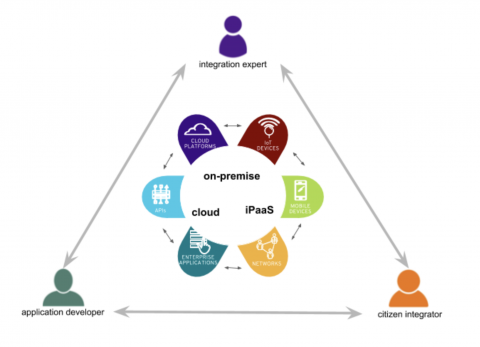
Red Hat Fuse is a distributed, cloud-native integration solution that has the flexibility to service diverse users - including integration experts, application developers, and business users - each with their own choice of deployment, architecture, and tooling. The result is an integration solution that supports collaboration across the enterprise.

High-level overview of Red Hat Fuse

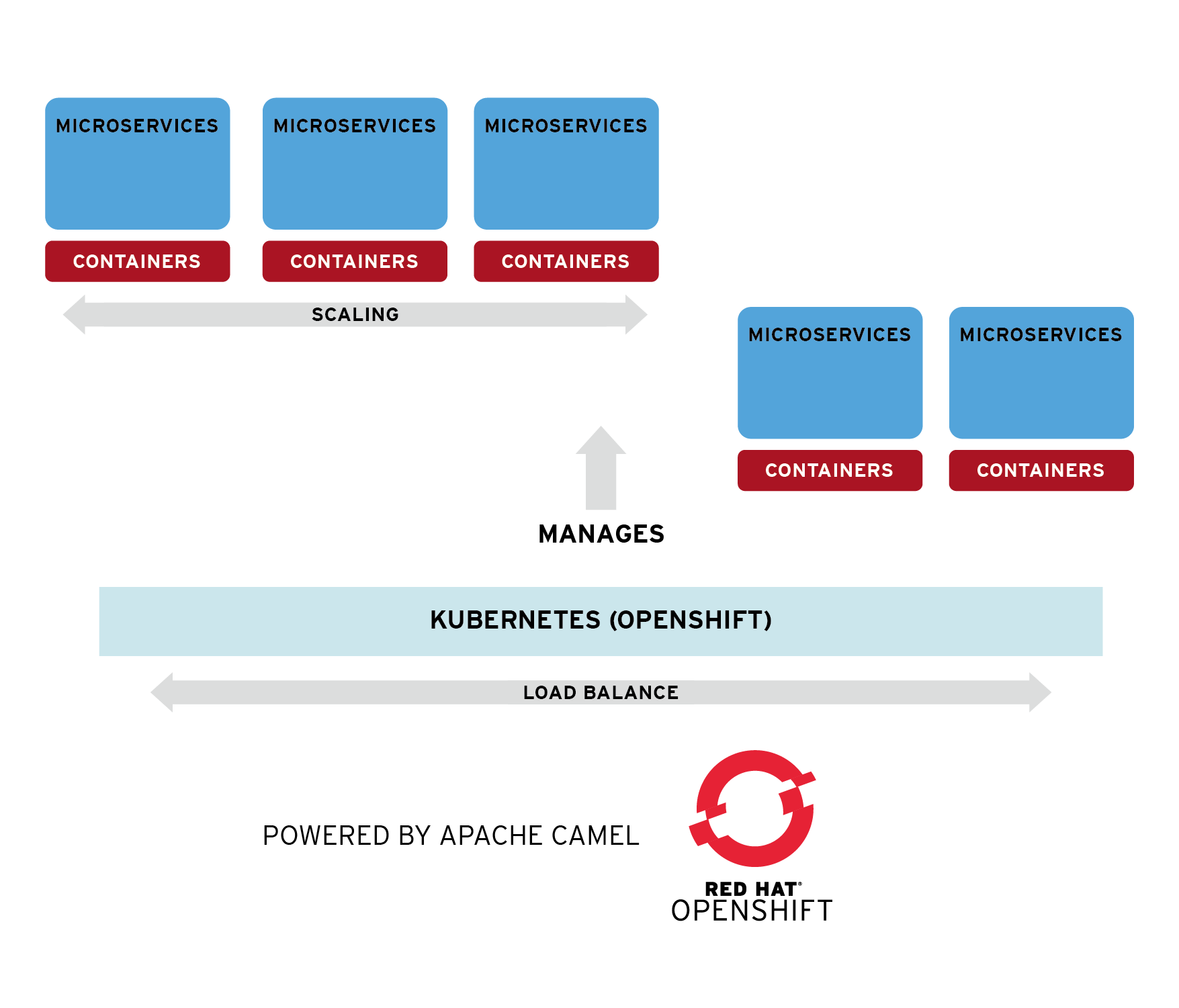
Red Hat Fuse enables developers to take an Agile Integration approach when developing solutions. By building and composing microservices, Fuse allows distributed systems deployments and a focus on scaling of services and people.

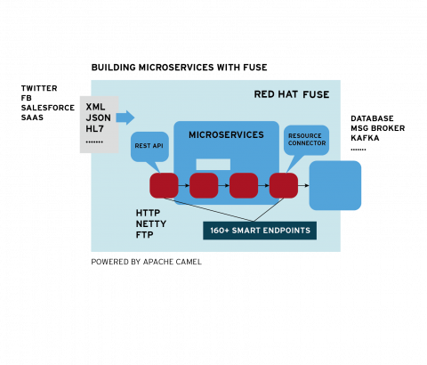
Distributed infrastructure Developing integration solution can be complex, and gets more hectic when the deployments are distributed on the cloud. Fuse, has its core integration capability based on the popular and versatile Apache Camel, provides predefined Enterprise Integration Patterns (EIPs) and over 200 connectors, are deployed on  container-native infrastructure to adapt easily and scale quickly.
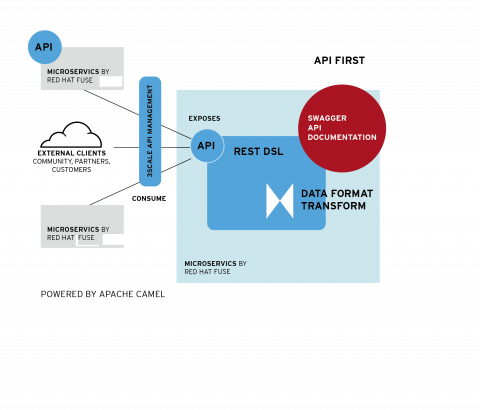
	Low-code interface Tooling allows developers and non-technical users to drag and drop predefined services and integration patterns so business units can self-serve and continuously innovative. API First Building an API-based architecture with Red Hat Fuse could not be easier. Red Hat Fuse is intuitive and simple to configure using Camel REST. Further, developers can design and document, RESTful APIs using Swagger technology for better collaboration. With Red Hat 3scale API Management, API security, performance, control and monetization are managed for you.
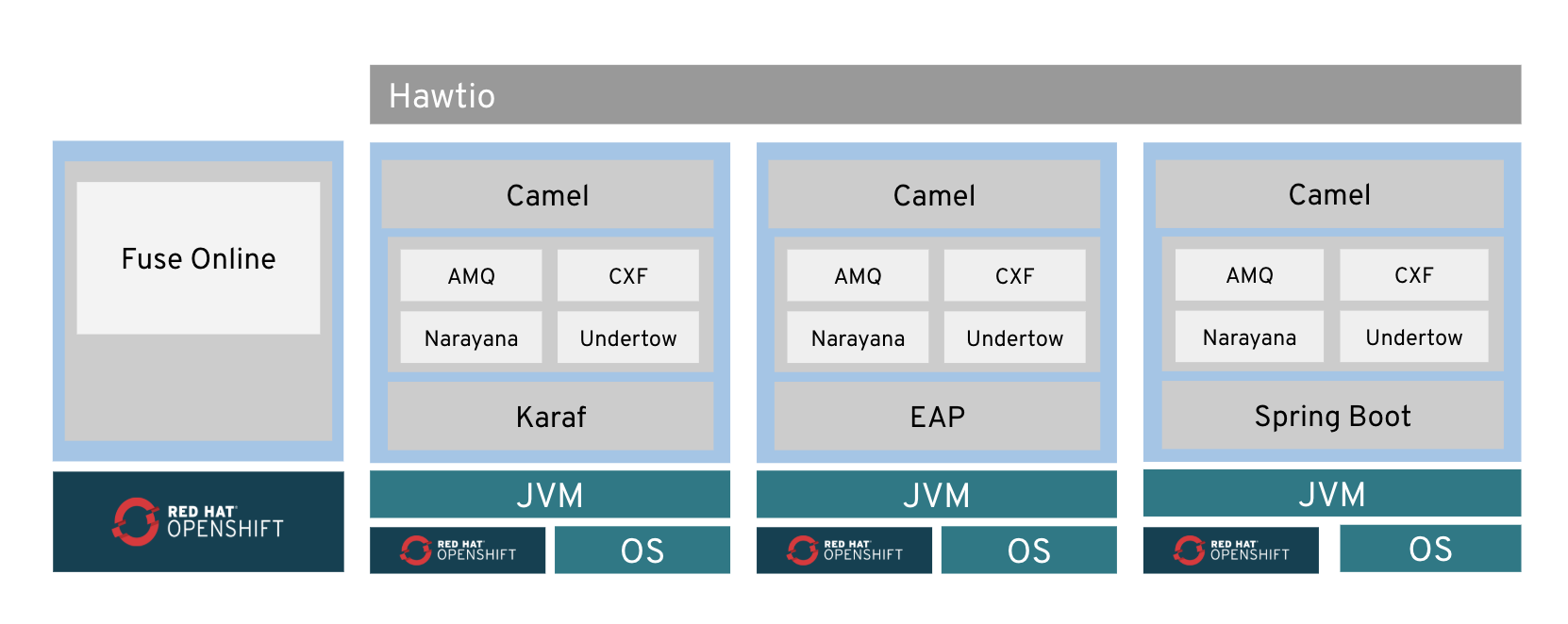
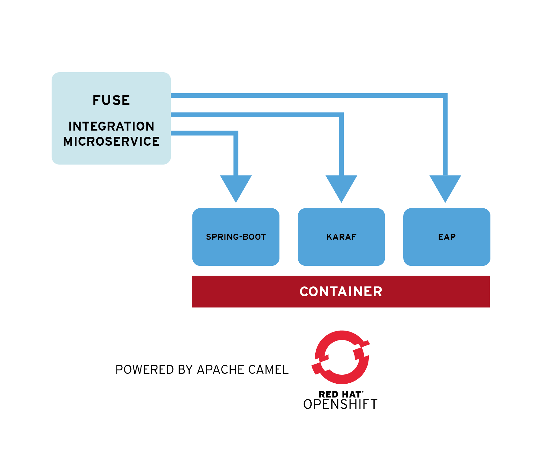
Container-Based Architecture With the freedom to develop and manage services in popular container standards -  including OSGI-based Apache Karaf, Java EE based JBoss EAP, and Spring-Boot. Fuse - you can package and deploy lightweight containers in distributed environments to allow for fault isolation and consistence settings.
	Continuous Improvement A simplified pipeline construction enables faster and safer software delivery. Jenkins allows for automatic testing, enable deployment and release best practices, and with native Continuous Integration and Deployment support, Fuse allows teams to work more collaboratively with faster software delivery. Hybrid Deployment  Use Red Hat Fuse on-prem, in public/private clouds, or as a hosted service and have all integration infrastructure work seamlessly together allowing users to collaborate across the enterprise.

inversion of control dependency injection design pattern spring example tutorial

Introduction to the Spring IoC container and beans

Spring Framework implementation of the Inversion of Control (IoC) ^[1]principle. IoC is also known as dependency injection (DI). It is a process whereby objects define their dependencies, that is, the other objects they work with, only through constructor arguments, arguments to a factory method, or properties that are set on the object instance after it is constructed or returned from a factory method. The container then injects those dependencies when it creates the bean. This process is fundamentally the inverse, hence the name Inversion of Control (IoC), of the bean itself controlling the instantiation or location of its dependencies by using direct construction of classes, or a mechanism such as the Service Locator pattern.

The org.springframework.beans and org.springframework.context packages are the basis for Spring Framework's IoC container. The BeanFactory interface provides an advanced configuration mechanism capable of managing any type of object. ApplicationContext is a sub-interface of BeanFactory. It adds easier integration with Spring's AOP features; message resource handling (for use in internationalization), event publication; and application-layer specific contexts such as the WebApplicationContext for use in web applications.

In short, the BeanFactory provides the configuration framework and basic functionality, and the ApplicationContext adds more enterprise-specific functionality. TheApplicationContext is a complete superset of the BeanFactory, and is used exclusively in this chapter in descriptions of Spring's IoC container. For more information on using the BeanFactory instead of the ApplicationContext, refer to Section 5.15, “The BeanFactory”.

In Spring, the objects that form the backbone of your application and that are managed by the Spring IoC container are called beans. A bean is an object that is instantiated, assembled, and otherwise managed by a Spring IoC container. Otherwise, a bean is simply one of many objects in your application. Beans, and the dependencies among them, are reflected in the configuration metadata used by a container.

5.2 Container overview

The interface org.springframework.context.ApplicationContext represents the Spring IoC container and is responsible for instantiating, configuring, and assembling the aforementioned beans. The container gets its instructions on what objects to instantiate, configure, and assemble by reading configuration metadata. The configuration metadata is represented in XML, Java annotations, or Java code. It allows you to express the objects that compose your application and the rich interdependencies between such objects.

Several implementations of the ApplicationContext interface are supplied out-of-the-box with Spring. In standalone applications it is common to create an instance of ClassPathXmlApplicationContext or FileSystemXmlApplicationContext. While XML has been the traditional format for defining configuration metadata you can instruct the container to use Java annotations or code as the metadata format by providing a small amount of XML configuration to declaratively enable support for these additional metadata formats.

In most application scenarios, explicit user code is not required to instantiate one or more instances of a Spring IoC container. For example, in a web application scenario, a simple eight (or so) lines of boilerplate J2EE web descriptor XML in the web.xml file of the application will typically suffice (see Section 5.14.4, “Convenient ApplicationContext instantiation for web applications”). If you are using the SpringSource Tool Suite Eclipse-powered development environment or Spring Roo this boilerplate configuration can be easily created with few mouse clicks or keystrokes.

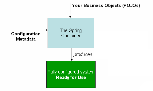
The following diagram is a high-level view of how Spring works. Your application classes are combined with configuration metadata so that after the ApplicationContext is created and initialized, you have a fully configured and executable system or application.

The Spring IoC container

Loading same class by two different class loader in java

here are, at least, two general ways to generate a ClassCastException under the conditions described. One is with a branched ClassLoader hierarchy, and the second is with a ClassLoader that does not preferentially delegate to its parent.
Read on for the long winded explanation ...

In a simple J2SE application (like "Hello World") there are at least three ClassLoader instances involved. In order (and order is very significant) these are:
1.) bootstrap classes,
2.) extension classes
3.) classpath (user) classes.
These form a hierarchy (parent-child relationship) where the child (higher number in the above list) class loaders delegate to their parent before trying to load a class themselves. The delegation behavior is by convention and is not enforced.
As long as this is a simple chain (one child per parent) and the contract for delegation is followed then ClassCastExceptions due to ClassLoader differences are impossible.
If the ClassLoader hierarchy branches (i.e. 2 or more children for any parent) then ClassCastExceptions may be thrown even if the class names are identical. This is the scenario illustrated in the earlier post by Mr Friedman-Hill where there are 2 instances of URLClassLoader, each a child of the classpath classloader.
Also, if a ClassLoader does not follow the convention of delegating first to its parent then the potential exists for ClassCastException due to different ClassLoader instances. The simplest way to do this would be to write a ClassLoader that loads a class before delegating to its parent, in which case it could load something that the parent already has loaded.
J2EE app servers use a ClassLoader hierarchy to enforce some security, e.g. not allowing EARs to access other EARs classes. The behavior depends on the app server. Some app servers use one ClassLoader per EAR and a child ClassLoader per WAR. Some use a sibling arrangement where a ClassLoader for a WAR delegates to a sibling classloader for an EJB-JAR.

A relavent reference from: http://java.sun.com/developer/technicalArticles/Networking/classloaders/index.html

"As of JDK 1.2, a bootstrap class loader that is built into the JVM is responsible for loading the classes of the Java runtime. This class loader only loads classes that are found in the boot classpath, and since these are trusted classes, the validation process is not performed as for untrusted classes. In addition to the bootstrap class loader, the JVM has an extension class loader responsible for loading classes from standard extension APIs, and a system class loader that loads classes from a general class path as well as your application classes.

Since there is more than one class loader, they are represented in a tree whose root is the bootstrap class loader. Each class loader has a reference to its parent class loader. When a class loader is asked to load a class, it consults its parent class loader before attempting to load the item itself. The parent in turn consults its parent, and so on. So it is only after all the ancestor class loaders cannot find the class that the current class loader gets involved. In other words, a delegation model is used.

why spring framework came in java?

Why Spring Framework?

Below is a chart given which shows the comparison between Spring and various other Frameworks.

It was named Interface 21, as a reference to 21st century and released under Apache 2.0 license.

This was the first milestone release. Spring framework rapidly evolved since this release. Interface21 supported AspectJ parallely with Spring Framework.

New Features were added – extensible XML configs, support for Java 5 and dynamic languages, IoC extension points and AOP enhancements.

New features were added – support for Java 6/ JEE5, annotation configs, component auto-detection in classpath and OSGi compliant bundles.

New features were added – support for reorganized module system, SpEL, JavaConfig, embedded databases, REST support and support for Java EE 6.

Spring Data Commons Project was released. Later in 2012, Rod Johnson left the Spring team.

All Spring projects shifted to Pivotal. New features were added – full support for Java 8, websockets, higher third party library dependencies, groovy DSL for bean definitions.

It was compatible with Java 6, 7 and 8, with a focus on core refinements and modern web capabilities.

It will be the final generation within the general Spring 4 system requirements. 4.3.8 is the current version.

Reasons for Spring Frameworks’s popularity




There are generally three main reasons for Spring Framework’s popularity.




Simplicity

Testablity

Loose Coupling

Let’s discuss these topics in details.




Simplicity: Spring Framework is simple because its non-invasive as it uses POJO and POJI models.<>




POJO (Plain Old Java Objects): A Java class not coupled with any technology or any framework is called “POJO”.

POJI (Plain Old Java Interfaces): A Java interface not coupled with any technology or any frame work is called “POJI”.

Testablity: For writing the Spring application, server is not mandatory. But for struts and EJB applications, you need a server, if you want to test the application. It may need lot of changes in the source and to view those changes, each time you have to restart the server. This becomes tedious and time consuming. In case of Spring Framework, it has it’s own container to run the applications.




Loose Coupling : Spring Framework is loosely coupled because it has concepts like Dependency Injection, AOP etc. These features help in reducing dependency and increasing the modularity within the code. Lets understand this with an example.




Here I have a Bike interface which has a start() method. It is further implemented by three classes, namely : Yamaha, Honda and Bajaj.

What is the difference between a Spring singleton and a Java singeleton(design pattern)?

The Java singleton is scoped by the Java class loader, the Spring singleton is scoped by the container context.

Which basically means that, in Java, you can be sure a singleton is a truly a singleton only within the context of the class loader which loaded it. Other class loaders should be capable of creating another instance of it (provided the class loaders are not in the same class loader hierarchy), despite of all your efforts in code to try to prevent it.

In Spring, if you could load your singleton class in two different contexts and then again we can break the singleton concept.

So, in summary, Java considers something a singleton if it cannot create more than one instance of that class within a given class loader, whereas Spring would consider something a singleton if it cannot create more than one instance of a class within a given container/context.